Characterizing a Functional Relationship Between Type 2 Diabetes and Alzheimer's disease With Mendelian Randomization
Introduction
In my last blogpost, I reviewed molecular pathways that are influental on Alzheimer's disease (AD) pathogenesis. The main pathway of my interest was PI3K/Akt pathway that is essential for neuronal growth, proliferation, cell survival, synaptic plasticity and cognitive function in central nervous system (CNS). This pathway is mediated by insulin signalling, impairment of which can lead to severe outcome in AD pathogenesis. Type 2 diabetes (T2D) is one major factor that contributes to impairment of insulin signalling, and also causes chronic systemic inflammation, which can furthermore attenuate AD disease progression.
AD is a complex disease and is a sum total of multiple factors, be it environmental, lifestyle or genetic. However, if taken proactive measures to diminish or outright remove some of these factors that cause AD, end result could be much more effective than starting the treatment once symptoms of AD present themselves. One measure could be altering one's lifestyle to diminish the individual's risk to develop AD. My point of interest is T2D, potentially major comorbidity factor to AD [1], and perhaps with proper diet, training and exercise, the risk of developing T2D could be nullified.
However, does T2D actually have functional connection with AD? This can be studied with observational study, where most common design is to control for confounding variables between the exposure and the outcome, but this strategy can easily lead to biased estimates and false conclusions [2]. Has relationship between AD and T2D been misled by confounding factors and is T2D not really causally related to AD, but associates with other factors that contribute to AD development? As chronic inflammation is associated with AD [3], regardless of T2D, could the causal relationship even be reversal, where AD is actually causing T2D? I'm interested in finding out, and with Mendelian randomization (MR) this could be possible!
Mendelian Randomization
MR utilizes the random assortment of parents genes to offspring during recombination, providing a method to assess the causal associations between exposure (in this case T2D) and outcome (in this case AD) [4, 5]. This method was originally coined with evaluating effectiveness of allogenic sibling bone marrow transplantation in treatment of acute myeloid leukaemia [6].
Human genome is enriched with single nucleotide polymorphisms (SNPs), where at a specific genomic locus, there can be a variation of single nucleotide from person to person, and these variations at specific loci create specific homozygous or heterozygous genotypes, determined by Mendelian heritability. If such SNPs produce phenotypic differences that mirror modifiable, disease risk altering environmental exposures, the different SNPs should be related to disease risk to the extent predicted by their influence on the phenotype [4].
Mendelian randomization has been propelled by the increasing availability and scale of genome-wide association studies (GWAS) summary data, and new meta-analysis methods have been developed around this data structure. However, if one doesn't plan the study accordingly, their study will make unrealistic simplifying assumptions and generally lack theoretical support such as statistical consistency and asymptotic sampling distribution results [2].
Mendelian Randomization With GWAS-Summary Data
I want to estimate the causal effect of an exposure variable X (T2D) on an outcome variable Y (AD), which may be confounded by unobserved variables. I have p amount of SNPs, that could be instrumental variables (IV), which can help me obtain unbiased estimate of the causal effect between T2D and AD, despite unmeasured confounding. The SNP-exposure effect and SNP-outcome effect can be computed from two different samples with linear or logistic regression [2].
With the assumption that for every SNP, the variances of The SNP-exposure effect and SNP-outcome are known and SNP-exposure effect and SNP-outcome are mutually independent, we can create a following model for GWAS summary data:
Γj ≈ β0 γj for almost all j ∈ [p]
Where Γj is the SNP-outcome effect, γj is the SNP-exposure effect, j represents a single SNP, [p] represents all SNPs and β0 is the outcome effect between X (T2D) on Y (AD) [2]. In order for the MR to be valid for testing causality, each specific SNP must be robustly associated with the exposure, independent of any confounders of the exposure and outcome, and be independent of the outcome given the exposure and the confounders (figure 1) [7].
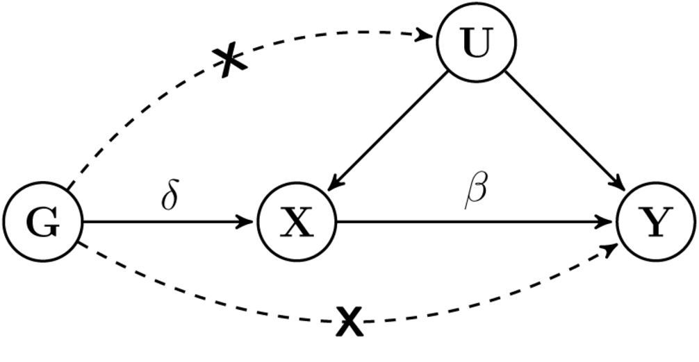
Figure 1. The general causal diagram and the three criteria for valid instrumental variable (IV). The diagram represents the hypothesized relationship between genetic instrument (G), exposure (X), outcome (Y) and all unmeasured variables (U) which confound X and Y. β is the causal effect of X on Y. δ is the genetic effect on X. Dashed lines and crosses indicate violations of the standard IV assumptions which can lead to bias [7].
MR-Base
Thankfully some streamlined tools have been made available to conduct MR experiments, such as MR-Base. MR-Base was developed to provide easy access to analysis-ready data and allow systematic application of Mendelian randomization methods. One convenient aspect about doing exposure-outcome assessment with MR-Base, is the accessibility of research data. MR-Base combines a database of summary statistics on traits and health outcomes from >20,000 GWAS datasets [5]. It is available as a web application or as an R package. I introduced myself to some handy tutorials, that made the installation and use of the tools a breeze.
Importing Libraries
In:
library (devtools)
install_github(c("MRCIEU/TwoSampleMR","MRCIEU/MRInstruments"))
# install_github("WSpiller/MRPracticals",build_opts = c("--no-resave-data", "--no-manual"),build_vignettes = FALSE) # useful tutorial vignettes for learning to use MR-Base
library(dplyr)
library(MRPracticals)
library(TwoSampleMR)
library(MRInstruments)
library(rsnps) # this is a handy tool for fetching metadata about discovered SNPs
get the GWAS data catalog and subset data
Here I'll fetch from NHGRI-EBI GWAS catalog of significant associations relevant datasets with "Type 2 diabetes" keyword in the phenotype_simple column. I'll also add European ancestry "EA" as inclusion criterion in the phenotype_info column.
In:
data("gwas_catalog")

# Using regular expressions can be handy in finding type 2 diabetes datasets, since there can be other vocabulary mixed in
exposure_gwas <- gwas_catalog[stringi::stri_detect_fixed(gwas_catalog$Phenotype_simple, "Type 2 diabetes"), ]

# EA = european ancestry
exposure_gwas <- subset(exposure_gwas, grepl("EA", Phenotype_info))

# Also, if one would be interested, it is also possible to select focus on either sex in the study,
# but I'm not going to implement that in this experiment

#exposure_gwas <- exposure_gwas[!grepl("women", exposure_gwas$Phenotype_info),]

#exposure_gwas <- exposure_gwas[!grepl("men", exposure_gwas$Phenotype_info),]
Preprocess and set parameters for exposure data
Let's inspect the dataset, and set p-value treshold, which in this case will be <5*10^-8. Setting the p-value treshold will ensure robust instruments.
In:
# set p-value treshold
exposure_gwas <- exposure_gwas[exposure_gwas$pval<5*10^-8,]

# format the data
exposure_data <- format_data(exposure_gwas)
Out:
other_allele column has some values that are not A/C/T/G or an indel comprising only these characters or D/I. These SNPs will be excludedMore than one type of unit specified for Type 2 diabetesThe following SNP(s) are missing required information for the MR tests and will be excluded
rs13266634
rs3923113
rs516946
rs7202877
rs7674212
rs7754840
rs7903146
rs944801
Also, I'll prune SNPs with clump_data function with linkage disequilibrium treshold value of 0.001. This will prune the set of SNPs for linkage disequilibrium, as using correlated SNPs can lead to biased causal effect estimates.
In:
# clump the gwas data based on LD
exposure_data <- clump_data(exposure_data, clump_r2 = 0.001)
Out:
API: public: http://gwas-api.mrcieu.ac.uk/
Please look at vignettes for options on running this locally if you need to run many instances of this command.
Clumping KoMTD8, 2 variants, using EUR population reference
Clumping x6K7fU, 24 variants, using EUR population reference
Removing 1 of 24 variants due to LD with other variants or absence from LD reference panel
Clumping KivTpa, 21 variants, using EUR population reference
Removing 1 of 21 variants due to LD with other variants or absence from LD reference panel
Fetching the Outcome Data
Here I'll fetch outcome datasets with the keyword "Alzheimer", from which I'll select a dataset, which has greatest number of SNPs. After this, I'll harmonize the data with harmonise_data function, where the effect of a SNP on the exposure and the effect of that SNP on the outcome must each correspond to the same allele.
In:
ao<-available_outcomes()
outcome_gwas <- subset(ao, grepl("Alzheimer", trait))
# pick GWAS outcome dataset, which has greatest nsnp value
highest_nsnp_count <- outcome_gwas %>% filter(nsnp == max(nsnp))
# fetch the outcome dataset
outcome_data <- extract_outcome_data(snps = exposure_data$SNP, outcomes = highest_nsnp_count[[1,1]])
Out:
Extracting data for 45 SNP(s) from 1 GWAS(s)
Finding proxies for 21 SNPs in outcome finn-a-G6_ALZHEIMER
Extracting data for 21 SNP(s) from 1 GWAS(s)
Do Mendelian randomization on harmonized data:
Because there are several id.exposure identificators, they create different groups in results, from which MR-Base creates several results. This can cause a flood of information. Therefore, I'll create a dplyr pipeline, which will select most numerous exposure by simply summing the number of each id.exposure and picking the one that is most numerous. harmonise_data function creates random identificators, so it will be easiest to pick the most numerous id.exposure this way.
In:
highest_count <- H_data %>% count(id.exposure) %>% filter(n == max(n))
highest_count
Out:
| id.exposure | n | |
|---|---|---|
| 1 | ctCHA2 | 20 |
In:
H_data2 <- subset(H_data, grepl(highest_count[1,1], id.exposure))
mr_results <- mr(H_data2)
mr_results
Out:
| id.exposure | id.outcome | outcome | exposure | method | nsnp | b | se | pval | |
|---|---|---|---|---|---|---|---|---|---|
| 1 | ctCHA2 | finn-a-G6_ALZHEIMER | Alzheimer disease || id:finn-a-G6_ALZHEIMER | Type 2 diabetes (unit decrease) | MR Egger | 20 | 0.36 | 0.41 | 0.40 |
| 2 | ctCHA2 | finn-a-G6_ALZHEIMER | Alzheimer disease || id:finn-a-G6_ALZHEIMER | Type 2 diabetes (unit decrease) | Weighted median | 20 | 0.19 | 0.16 | 0.24 |
| 3 | ctCHA2 | finn-a-G6_ALZHEIMER | Alzheimer disease || id:finn-a-G6_ALZHEIMER | Type 2 diabetes (unit decrease) | Inverse variance weighted | 20 | 0.30 | 0.11 | 0.01 |
| 4 | ctCHA2 | finn-a-G6_ALZHEIMER | Alzheimer disease || id:finn-a-G6_ALZHEIMER | Type 2 diabetes (unit decrease) | Simple mode | 20 | 0.09 | 0.27 | 0.75 |
| 5 | ctCHA2 | finn-a-G6_ALZHEIMER | Alzheimer disease || id:finn-a-G6_ALZHEIMER | Type 2 diabetes (unit decrease) | Weighted mode | 20 | 0.14 | 0.25 | 0.59 |
Reviewing the Results
Let's see the odds ratio scale if there is any statistically significant relationship between T2D and AD.
In:
generate_odds_ratios(mr_results)
Out:
| id.exposure | id.outcome | outcome | exposure | method | nsnp | b | se | pval | lo_ci | up_ci | or | or_lci95 | or_uci95 | |
|---|---|---|---|---|---|---|---|---|---|---|---|---|---|---|
| 1 | ctCHA2 | finn-a-G6_ALZHEIMER | Alzheimer disease || id:finn-a-G6_ALZHEIMER | Type 2 diabetes (unit decrease) | MR Egger | 20 | 0.36 | 0.41 | 0.40 | -0.45 | 1.17 | 1.43 | 0.64 | 3.21 |
| 2 | ctCHA2 | finn-a-G6_ALZHEIMER | Alzheimer disease || id:finn-a-G6_ALZHEIMER | Type 2 diabetes (unit decrease) | Weighted median | 20 | 0.19 | 0.16 | 0.24 | -0.13 | 0.50 | 1.21 | 0.88 | 1.66 |
| 3 | ctCHA2 | finn-a-G6_ALZHEIMER | Alzheimer disease || id:finn-a-G6_ALZHEIMER | Type 2 diabetes (unit decrease) | Inverse variance weighted | 20 | 0.30 | 0.11 | 0.01 | 0.08 | 0.51 | 1.34 | 1.08 | 1.67 |
| 4 | ctCHA2 | finn-a-G6_ALZHEIMER | Alzheimer disease || id:finn-a-G6_ALZHEIMER | Type 2 diabetes (unit decrease) | Simple mode | 20 | 0.09 | 0.27 | 0.75 | -0.44 | 0.61 | 1.09 | 0.64 | 1.85 |
| 5 | ctCHA2 | finn-a-G6_ALZHEIMER | Alzheimer disease || id:finn-a-G6_ALZHEIMER | Type 2 diabetes (unit decrease) | Weighted mode | 20 | 0.14 | 0.25 | 0.59 | -0.35 | 0.63 | 1.15 | 0.70 | 1.87 |
Only inverse variance weighted (IVW) method gave p-value of ~0.007. IVW method calculates the Wald ratio for each of the instruments and combines the results using an inverse-variance weighted meta-analysis approach. The slope from this approach can be interpreted as the causal effect of the exposure on the outcome. With mr_pleiotropy_test, we can review MR-Egger regression intercept, which provides an estimate of the magnitude of horizontal pleiotropy.
In:
mr_pleiotropy_test(H_data2)
mr_heterogeneity(H_data2, method_list=c("mr_egger_regression", "mr_ivw"))
Out:
| id.exposure | id.outcome | outcome | exposure | method | Q | Q_df | Q_pval | |
|---|---|---|---|---|---|---|---|---|
| 1 | ctCHA2 | finn-a-G6_ALZHEIMER | Alzheimer disease || id:finn-a-G6_ALZHEIMER | Type 2 diabetes (unit decrease) | MR Egger | 17.00 | 18.00 | 0.52 |
| 2 | ctCHA2 | finn-a-G6_ALZHEIMER | Alzheimer disease || id:finn-a-G6_ALZHEIMER | Type 2 diabetes (unit decrease) | Inverse variance weighted | 17.02 | 19.00 | 0.59 |
Plotting the Results
mr_scatter_plot function produces method comparison plot, that is a graphical representation of the effect of the SNPs on the exposure, that is always positive and the effect of the SNPs on the outcome is directed accordingly. I'll inspect individual SNP effects with forest plots and leave-one-out plots. Lastly, I'll depict a funnel plot, which presents the effect estimates against a measure of precision, which in this case will give visual assessment of heterogeneity.
In:
res_singles <- mr_singlesnp(H_data2)
res_loo <- mr_leaveoneout(H_data2)
mr_funnel <- mr_funnel_plot(res_singles)

mr_scatter_plot(mr_results, H_data2)
Out:

Figure 2. Method comparison plot. Indicates some minor effect exposure-outcome effect between T2D and AD.
Forest plots depict summary graphs showing the individual effects of SNPs, calculated using the Wald ratio, along with the overall results to assess the consistency across SNPs.
In:
mr_forest_plot(res_singles)Out:

Figure 3. Forest plot of causal effects of individual SNPs to the outcome.
Leave-one-out graph shows the results of MR analyses using the IVW method when leaving one SNP out each time. This analysis can be used to assess whether the SNPs are consistent in terms of their effect on the overall outcome or whether the results are being driven by a single outlying SNP.
In:
mr_leaveoneout_plot(res_loo)Out:

Figure 4. Leave-one-out analysis plot.
Horizontal pleiotropy occurs when the outcome is affected by the SNPs through a pathway that is independent of the exposure and invalidates the second Mendelian randomization assumption. A funnel plot can be used to assess heterogeneity, particularly horizontal pleiotropy, which is likely if points are spread. Directional horizontal pleiotropy may be present if the graph is not symmetrical. If the spread is weighted toward certain direction, this can be evidence of directional pleiotropy.
In:
mr_funnel_plot(res_singles)Out:

Figure 5. Funnel plot visually to assess heterogeneity.
Query SNP Data
It thought it would handy, if the script would also automatically return a report about the SNPs presented in the forest plot. This would make inspecting SNPs much simpler, since the user doesn't necessarily have search from external sources metadata concerning these SNPs.
In:
snps <- res_singles$SNP[1:as.numeric(length(res_singles$SNP)-2)]
ncbi_snp_query(snps)
Out:
| query | chromosome | bp | class | rsid | gene | alleles | ancestral_allele | variation_allele | seqname | hgvs | assembly | ref_seq | minor | maf | |
|---|---|---|---|---|---|---|---|---|---|---|---|---|---|---|---|
| 1 | rs10811661 | 9 | 22134095.00 | snv | rs10811661 | T,A,C | T | A,C | NC_000009.12 | NC_000009.12:g.22134095T>A,NC_000009.12:g.22134095T>C | GRCh38.p12 | T | C | 0.14 | |
| 2 | rs1111875 | 10 | 92703125.00 | snv | rs1111875 | C,G,T | C | G,T | NC_000010.11 | NC_000010.11:g.92703125C>G,NC_000010.11:g.92703125C>T | GRCh38.p12 | C | T | 0.38 | |
| 3 | rs11708067 | 3 | 123346931.00 | snv | rs11708067 | ADCY5 | A,G | A | G | NC_000003.12 | NC_000003.12:g.123346931A>G | GRCh38.p12 | A | G | 0.18 |
| 4 | rs12571751 | 10 | 79182874.00 | snv | rs12571751 | ZMIZ1 | A,G | A | G | NC_000010.11 | NC_000010.11:g.79182874A>G | GRCh38.p12 | A | G | 0.47 |
| 5 | rs13266634 | 8 | 117172544.00 | snv | rs13266634 | SLC30A8/LOC105375716 | C,A,T | C | A,T | NC_000008.11 | NC_000008.11:g.117172544C>A,NC_000008.11:g.117172544C>T | GRCh38.p12 | C | T | 0.27 |
| 6 | rs1552224 | 11 | 72722053.00 | snv | rs1552224 | ARAP1 | A,C | A | C | NC_000011.10 | NC_000011.10:g.72722053A>C | GRCh38.p12 | A | C | 0.13 |
| 7 | rs1801282 | 3 | 12351626.00 | snv | rs1801282 | PPARG | C,G | C | G | NC_000003.12 | NC_000003.12:g.12351626C>G | GRCh38.p12 | C | G | 0.10 |
| 8 | rs2237892 | 11 | 2818521.00 | snv | rs2237892 | KCNQ1 | C,T | C | T | NC_000011.10 | NC_000011.10:g.2818521C>T | GRCh38.p12 | C | T | 0.09 |
| 9 | rs2421016 | 10 | 122407996.00 | snv | rs2421016 | PLEKHA1 | C,T | C | T | NC_000010.11 | NC_000010.11:g.122407996C>T | GRCh38.p12 | C | T | 0.48 |
| 10 | rs2796441 | 9 | 81694033.00 | snv | rs2796441 | LOC101927502 | G,A,T | G | A,T | NC_000009.12 | NC_000009.12:g.81694033G>A,NC_000009.12:g.81694033G>T | GRCh38.p12 | G | A | 0.35 |
| 11 | rs3923113 | 2 | 164645339.00 | snv | rs3923113 | A,C,G,T | A | C,G,T | NC_000002.12 | NC_000002.12:g.164645339A>C,NC_000002.12:g.164645339A>G,NC_000002.12:g.164645339A>T | GRCh38.p12 | A | C | 0.43 | |
| 12 | rs4457053 | 5 | 77129124.00 | snv | rs4457053 | ZBED3-AS1 | G,A | G | A | NC_000005.10 | NC_000005.10:g.77129124G>A | GRCh38.p12 | G | A | 0.76 |
| 13 | rs4607103 | 3 | 64726228.00 | snv | rs4607103 | ADAMTS9-AS2 | C,G,T | C | G,T | NC_000003.12 | NC_000003.12:g.64726228C>G,NC_000003.12:g.64726228C>T | GRCh38.p12 | C | T | 0.27 |
| 14 | rs5215 | 11 | 17387083.00 | snv | rs5215 | KCNJ11 | C,T | C | T | NC_000011.10 | NC_000011.10:g.17387083C>T | GRCh38.p12 | C | T | 0.70 |
| 15 | rs7202877 | 16 | 75213347.00 | snv | rs7202877 | T,C,G | T | C,G | NC_000016.10 | NC_000016.10:g.75213347T>C,NC_000016.10:g.75213347T>G | GRCh38.p12 | ||||
| 16 | rs7578326 | 2 | 226155937.00 | snv | rs7578326 | LOC646736 | A,G | A | G | NC_000002.12 | NC_000002.12:g.226155937A>G | GRCh38.p12 | A | G | 0.35 |
| 17 | rs7578597 | 2 | 43505684.00 | snv | rs7578597 | THADA | T,C | T | C | NC_000002.12 | NC_000002.12:g.43505684T>C | GRCh38.p12 | T | C | 0.13 |
| 18 | rs7957197 | 12 | 121022883.00 | snv | rs7957197 | OASL | T,A | T | A | NC_000012.12 | NC_000012.12:g.121022883T>A | GRCh38.p12 | T | A | 0.18 |
| 19 | rs864745 | 7 | 28140937.00 | snv | rs864745 | JAZF1 | T,C | T | C | NC_000007.14 | NC_000007.14:g.28140937T>C | GRCh38.p12 | T | C | 0.42 |
| 20 | rs9505118 | 6 | 7290204.00 | snv | rs9505118 | SSR1 | A,G | A | G | NC_000006.12 | NC_000006.12:g.7290204A>G | GRCh38.p12 | A | G | 0.37 |
Discussion
Unfortunately, the results are quite inconsistent, and only inverse variance weighted (IVW) method gave p-value of ~0.007. Other methods present non-significant causal effect between T2D and AD, that may be the result from too small number of SNPs in my dataset, too differing ethnic background between exposure and outcome datasets, or there isn't significant causal relationship between T2D and AD and there may may be bias in IVW method.
Method comparison plot depicted some exposure-outcome effect between T2D and AD, but the different method regressions spread out as the magnitude increased, indicating non-constant variability in the measurement. Pleiotropy levels were ~-0.0057 (SE: ~0.037, p = ~0.88). Thus, MR-Egger intercept was not significant using a 95% threshold, neither there was any heterogeneity between individual SNP estimates at a global level, which was indicated by the Q statistics and corresponding p-values for heterogeneity. This was further supported by funnel plot, which, compared to examples [5], doesn't have too wide spread, and also seems symmetrical. However, the relatively small number of SNPs leave some room for speculation.
Overall, these results don't have the final say on causal relationship between T2D and AD, but it was a good exercise in using R and MR-Base.
Sources
- Jayaraman A, Pike CJ. Alzheimer's disease and type 2 diabetes: multiple mechanisms contribute to interactions. Curr Diab Rep. 2014;14(4):476. doi:10.1007/s11892-014-0476-2
- Zhao, Q. et al. Statistical inference in two-sample summary-data Mendelian randomization using robust adjusted profile score. arXiv:1801.09652v3
- Kinney JW et al. Inflammation as a central mechanism in Alzheimer's disease. Alzheimers Dement (N Y). 2018;4:575-590. Published 2018 Sep 6. doi:10.1016/j.trci.2018.06.014
- Smith GD, Ebrahim S. 'Mendelian randomization': can genetic epidemiology contribute to understanding environmental determinants of disease? Int J Epidemiol. 2003 Feb;32(1):1-22. doi: 10.1093/ije/dyg070. PMID: 12689998.
- Walker VM et al. Using the MR-Base platform to investigate risk factors and drug targets for thousands of phenotypes. Wellcome Open Res. 2019;4:113. Published 2019 Nov 7. doi:10.12688/wellcomeopenres.15334.2
- Gray R, Wheatley K. How to avoid bias when comparing bone marrow transplantation with chemotherapy. Bone Marrow Transplant. 1991;7 Suppl 3:9-12. PMID: 1855097.
- Shapland CY et al. Profile-likelihood Bayesian model averaging for two-sample summary data Mendelian randomization in the presence of horizontal pleiotropy. bioRxiv 2020.02.11.943712; doi: https://doi.org/10.1101/2020.02.11.943712
Back to home page