Causal Association Between T2D & AD with MR

In this notebook, we will demonstrate Two-Sample Mendelian Randomisation (2SMR) pipeline with TwoSampleMR R library. We shall investigate causal effect of type 2 diabetes (T2D) on Alzheimer’s disease (AD). For exposure dataset, FinnGen data freeze 4 E4_DM2_STRICT (type 1 diabetes as exclusion restriction and Type 2 diabetes with coma, ketoacidosis, renal complications, ophthalmic complications, neurological complications, peripheral circulatory complications, other complications, and without complications as inclusion restriction) GWAS summary-level statistics dataset, with 23 338 cases and 148 190 controls of Finnish ancestry was used (FinnGen, 2020). For outcome dataset, Jansen et al. 24 087 European ancestry late-onset Alzheimer’s disease cases, 47,793 UK Biobank European ancestry individuals with family history of Alzheimer’s disease (AD-by-proxy), which is based on parental diagnoses, showed strong genetic correlation with AD (rg = 0.81), and 383 378 European ancestry controls was used (Jansen et al., 2019).

library(devtools)

## Loading required package: usethis

library(dplyr)

## 
## Attaching package: 'dplyr'

## The following objects are masked from 'package:stats':
## 
##     filter, lag

## The following objects are masked from 'package:base':
## 
##     intersect, setdiff, setequal, union

#devtools::install_github("MRCIEU/TwoSampleMR")
library(TwoSampleMR)

## TwoSampleMR version 0.5.5 
## [>] New: Option to use non-European LD reference panels for clumping etc
## [>] Some studies temporarily quarantined to verify effect allele
## [>] See news(package='TwoSampleMR') and https://gwas.mrcieu.ac.uk for further details

## 
## Warning:
## You are running an old version of the TwoSampleMR package.
## This version:   0.5.5
## Latest version: 0.5.6
## Please consider updating using devtools::install_github('MRCIEU/TwoSampleMR')

#devtools::install_github("jyypma/nloptr")
library(simex)
library(xlsx)

Set Parameters

First, we will set working directory as TwoSampleMR. dir.create() does not cause a crash if the directory already exists, it just prints out a warning.

dir.create("TwoSampleMR")
setwd("TwoSampleMR")

After that, we will set download url addressess for exposure and outcome datasets, after which we’ll set set phenocodes for our datasets, which will determine the names for exported files and their directory.

Getting Finngen datasets is very easy, since you can just change phenocode variable and don’t have to worry about dataset variable naming, since they are the same across all R4 Finngen GWAS summary statistics datasets.

Few phenocode examples:

E4_DM2OPTH – Type 2 diabetes with ophthalmic complications
AD_LO – Alzheimer’s disease (Late onset)
C3_PROSTATE – Malignant neoplasm of prostate

A direct download of comprehensive list of Finngen R4 endpoints is available in this link (accessed 30.3.2021).

url1 <- "https://storage.googleapis.com/finngen-public-data-r4/summary_stats/finngen_R4_"
url2 <- "ftp://ftp.ebi.ac.uk/pub/databases/gwas/summary_statistics/JansenIE_30617256_GCST007320/"
expPhenocode <- "E4_DM2_STRICT"
outPhenocode <- "AD_sumstats_Jansenetal_2019sept"

expFileEnd <- ".gz"
outFileEnd <- ".txt.gz"

expFilename <- paste(expPhenocode, ".tsv", sep="")
outFilename <- paste(outPhenocode, ".tsv", sep="")
resultsName <- paste(expPhenocode, "_VS_", outPhenocode, sep="")

dir.create(resultsName)
setwd(resultsName)

And lastly, we will set exposure variant p-value filtering as 5*10^-8, linkage disequilibrium (LD) clumping as 0.001, and pruning method parameter as 1. When pruning method set to 1, the duplicate summary sets are first dropped on the basis of the outcome sample size (smaller duplicates dropped).

If you are using power.prune function, when method is set to 2, duplicates are dropped on the basis of instrument strength (amount of variation explained in the exposure by the instrumental variables) and sample size, and assumes that the genetic variant-exposure effects correspond to a continuous trait with a normal distribution. However, in this study power pruning had no effect in the total number of genetic variants, so it was omitted.

We will set mendelian randomization methods into a list_of_mr_methods vector variable. A recommendation is to perform the MR-Egger, median-based method, and mode-based method, as these methods require different assumptions to be satisfied for asymptotically consistent estimates. Different methods will perform better and worse in different scenarios, so critical thought and judgement is required.

pval <- 5*10^-8

# I've set three r^2 thresholds for setting up a stepwise LD 
clump1 <- 0.1
clump2 <- 0.2
clump3 <- 0.4

# Prune method 1 for binary outcome
prune_method <- 1

# five different estimators for MR analysis
list_of_mr_methods<-c("mr_ivw", "mr_egger_regression") 
                     #"mr_weighted_median",
                     #"mr_weighted_mode")

# assign exposure and outcome cases and controls
exposureCases <- 23338
exposureControls <- 148190 - exposureCases
outcomeCases <- 24087 + 47793
outcomeControls <- 383378

Import Exposure Data

In the following cell, we will download the exposure dataset with chaining url string variable and phenocode, from which we get the complete url address to download the dataset summary GWAS dataset repository. Because the TwoSampleMR cannot read dataframe variables as input, we have to save the dataframes into the working directory as .tsv-files.

import_data <- function(url, phenocode, cases, controls, filename) {
  
  tmp <- tempfile()
  
  # here we check if there is .gz in the url address, if there is, then the downloaded file will be unzipped
  if (grepl("^.*(.gz)[[:space:]]*$", paste(url1, phenocode, sep="")) == TRUE) {
    download.file(paste(url, phenocode, sep=""), tmp)
  
    # unzipping the .gz file and reading it into a dataframe
    dat <- read.csv(
      gzfile(tmp),
      sep="\t",
      header=TRUE,
      stringsAsFactors = FALSE
      )
  } else {
    download.file(paste(url, phenocode, sep=""), tmp)
    
      dat <- read.csv(
      tmp,
      sep="\t",
      header=TRUE,
      stringsAsFactors = FALSE
      )
  }
  
  # adding a phenocode column, makes data identification easier
  dat["phenocode"] <- phenocode
  
  dat["cases"] <- cases
  dat["controls"] <- controls
  sampleSize <- cases + controls
  dat["sampleSize"] <- sampleSize
  
  return(dat)

}

exposure_df <- import_data(url1, paste0(expPhenocode, expFileEnd, sep=""), exposureCases, exposureControls, expFilename)
outcome_df <- import_data(url2, paste0(outPhenocode, outFileEnd, sep=""), outcomeCases, outcomeControls, outFilename)

Reading In the GWAS Summary Datasets For TwoSampleMR

In the following cell, we will read exposure and outcome dataframes into proper format with format_data function. This can be tricky if you cannot get the column names right. Since the standards are quite lax for GWAS summary dataset column naming. One should check the dataset columns and identify the right ones before inputing them into the read_exposure_data, read_outcome_data, or format_data functions. .tsv files from local repository can be read with TwoSampleMRs read_exposure_data and read_outcome_data functions.

# This function is for formatting the downloaded dataframe stored in R global environment 
exposure_gwas <- format_data(
  exposure_df,
  type = "exposure",
  snps = NULL,
  header = TRUE,
  phenotype_col = "phenocode",
  snp_col = "rsids",
  beta_col = "beta",
  se_col = "sebeta",
  eaf_col = "maf",
  effect_allele_col = "ref",
  other_allele_col = "alt",
  pval_col = "pval",
  ncase_col = "cases",
  ncontrol_col = "controls",
  samplesize_col = "sampleSize",
  gene_col = "nearest_genes",
  min_pval = 1e-200,
  log_pval = FALSE
)

outcome_gwas <- format_data(
  outcome_df,
  type = "outcome",
  snps = NULL,
  header = TRUE,
  phenotype_col = "phenocode",
  snp_col = "SNP",
  beta_col = "BETA",
  se_col = "SE",
  eaf_col = "EAF",
  effect_allele_col = "A1",
  other_allele_col = "A2",
  pval_col = "P",
  ncase_col = "cases",
  ncontrol_col = "controls",
  samplesize_col = "sampleSize",
  gene_col = "uniqID.a1a2",
  min_pval = 1e-200,
  log_pval = FALSE
)

Data Harmonisation and Export

In 2SMR, appropriate data harmonization is essential when combining two independently generated datasets, since GWAS results rarely have harmonized effect alleles. First, we will define a get_H_data function that takes in exposure and outcome GWAS summary datasets, p-value threshold, clump value and pruning method as parameters. This function will filter exposure dataset saving genetic variants that have p-value lower than the threshold.

Then, we will select independent SNPs with ‘clumping’, which identifies independent signals by considering the LD between SNPs. LD-association may skew the causal estimation, so with least squares correlation estimate, they can be filtered. In this example, we’ll implement stepwise thresholds of 0.1, 0.2 and 0.4, just to get an idea if LD-thresholding has an effect on horizontal pleiotropy.

With harmonise_data function, we will use the default action parameter value that tries to infer positive strand alleles, using allele frequencies for palindromes.

When there are duplicate summary sets for a particular exposure-outcome combination, power_prune keeps the exposure-outcome summary set with the highest expected statistical power. This can be done by dropping the duplicate summary sets with the smaller sample sizes. Alternatively, the pruning procedure can take into account instrument strength and outcome sample size. The latter is useful, for example, when there is considerable variation in SNP coverage between duplicate summary sets (e.g. because some studies have used targeted or fine mapping arrays). If there are a large number of SNPs available to instrument an exposure, the outcome GWAS with the better SNP coverage may provide better power than the outcome GWAS with the larger sample size. If the exposure is binary then method=1 should be used. However, this function is omitted from this pipeline, since it has no effect in the final dataset.

In addition, in this part it may be most prudent choice to export harmonized datasets. Since some genetic variants, which may violate IV assumptions 2 and 3 through biological mechanisms, can be discounted before the harmonized dataset is inputed to MR analysis.

get_H_data <- function(exposure_gwas, outcome_gwas, pvalue, clump_value, prune_method) {
  
  # filter based on p-value threshold
  exposure_gwas2 <- exposure_gwas[as.numeric(exposure_gwas$pval.exposure)<pvalue,]
  
  # check if we got any 
  print(paste0("before clumping ",dim(exposure_gwas2)))
  # clump the gwas data based on LD
  exposure_gwas2 <- clump_data(exposure_gwas2, clump_r2 = clump_value)
  print(paste0("before harmonizing ",dim(exposure_gwas2)))
  H_data <- harmonise_data(exposure_dat = exposure_gwas2, outcome_dat = outcome_gwas)
  
  # H_data power pruning is omitted from this experiment, since it doesn't affect the resulting amount of genetic variants
  #print(paste0("before power pruning ",dim(H_data)))
  #H_data<-power_prune(H_data, method = prune_method, dist.outcome = "binary")
  
  #print(paste0("after power pruning ",dim(H_data)))
  
  #H_data <- add_rsq(H_data)
  return(H_data)
}

# exposure, outcome, log-p-value, clump value, power prune method
H_data1 <- get_H_data(exposure_gwas, outcome_gwas, pval, clump1, prune_method)

## [1] "before clumping 1477" "before clumping 16"

## API: public: http://gwas-api.mrcieu.ac.uk/

## Please look at vignettes for options on running this locally if you need to run many instances of this command.

## Clumping K85KuF, 1477 variants, using EUR population reference

## Removing 1410 of 1477 variants due to LD with other variants or absence from LD reference panel

## [1] "before harmonizing 67" "before harmonizing 16"

## Harmonising E4_DM2_STRICT.gz (K85KuF) and AD_sumstats_Jansenetal_2019sept.txt.gz (RtsVCl)

H_data2 <- get_H_data(exposure_gwas, outcome_gwas, pval, clump2, prune_method)

## [1] "before clumping 1477" "before clumping 16"

## Please look at vignettes for options on running this locally if you need to run many instances of this command.

## Clumping K85KuF, 1477 variants, using EUR population reference

## Removing 1399 of 1477 variants due to LD with other variants or absence from LD reference panel

## [1] "before harmonizing 78" "before harmonizing 16"

## Harmonising E4_DM2_STRICT.gz (K85KuF) and AD_sumstats_Jansenetal_2019sept.txt.gz (RtsVCl)

H_data3 <- get_H_data(exposure_gwas, outcome_gwas, pval, clump3, prune_method)

## [1] "before clumping 1477" "before clumping 16"

## Please look at vignettes for options on running this locally if you need to run many instances of this command.

## Clumping K85KuF, 1477 variants, using EUR population reference

## Removing 1376 of 1477 variants due to LD with other variants or absence from LD reference panel

## [1] "before harmonizing 101" "before harmonizing 16"

## Harmonising E4_DM2_STRICT.gz (K85KuF) and AD_sumstats_Jansenetal_2019sept.txt.gz (RtsVCl)

# export harmonized datasets to save a list of IVs before pruning pleiotropic genes
# IV assumptions through biological mechanisms
write.csv(H_data1, paste(resultsName, "H_data01.csv"))
write.csv(H_data2, paste(resultsName, "H_data02.csv"))
write.csv(H_data3, paste(resultsName, "H_data04.csv"))

Import H_data (if you already have harmonized datasets in your working directory)

The following cell is only for importing harmonized data from local repository. If you wish to perform a 2SMR analysis on already harmonized datasets, you can import them with following simple commands.

#H_data1 <- read.csv("some_harmonized_gwas_data_01.csv")
#H_data2 <- read.csv("some_harmonized_gwas_data_02.csv")
#H_data3 <- read.csv("some_harmonized_gwas_data_03.csv")

Remove Rows Based on Gene

Here we discount genetic variants, referring to a “discountable” vector, with which we filter discountable genes from the dataframe. If one does not have gene names incorptorated into their gwas dataset, then they can refer to the genetic variant rs ID instead, and refer to the SNP column instead of the gene.exposure column.

filter_IVs <- function(H_data, gene_vector){
for (gene in gene_vector){
  H_data <- H_data[!grepl(gene, H_data$gene.exposure),] 
  }
  return(H_data)
}

# assign genes that will be used to filter genetic variants associated with potentially pleiotropic genes
# You can switch these with genetic variant rs ids, if you want to be more specific with which genetic variant you want to discount
discountable <- c("JAZF1", "WFS1", "MTNR1B", "HHEX", "UBE2G1", "PPARG", 
                "TCF7L2", "IRS1", "CDKAL1", "THADA", "IGF2BP2", "ZBED3", 
                "ADCY5", "FTO")


# if you are filtering genetic variants based on rs id instead of gene names, change gene.exposure column to SNP in the filter_IVs function!
filtered_H_data1 <- filter_IVs(H_data1, discountable)
filtered_H_data2 <- filter_IVs(H_data2, discountable)
filtered_H_data3 <- filter_IVs(H_data3, discountable)

QC-check

A strong positive correlation that is less than 1 (i.e. partial LD) implies that the effect alleles of the target and the LD proxy variants are typically in phase, but not necessarily due to recombination events. We will also check if there are any allele mismatches and effect allele frequency values that are close to 0.5. These SNPs require that the effect allele frequency is reported, and that the minor allele frequency is substantially below 50% in order to identify ambiguities. This code snippet essentially just double checks TwoSampleMR’s harmonization results. If this produces empty dataframes, then the harmonization should be good.

QCcheck <- function(H_data){
  print(H_data[H_data$effect_allele.exposure != H_data$effect_allele.outcome])
  print(H_data[H_data$other_allele.outcome != H_data$other_allele.exposure])
  
  exweak<-H_data %>% filter(H_data$eaf.exposure > 0.45, H_data$eaf.exposure < 0.55)
  print(paste("SNP with effect allele frequency close to 0.5: ", exweak$SNP, " palindromic: ", exweak$palindromic))
  return(exweak)
}

exweak1 <- QCcheck(filtered_H_data1)

## data frame with 0 columns and 41 rows
## data frame with 0 columns and 41 rows
## [1] "SNP with effect allele frequency close to 0.5:  rs10938397  palindromic:  FALSE"
## [2] "SNP with effect allele frequency close to 0.5:  rs11668971  palindromic:  FALSE"
## [3] "SNP with effect allele frequency close to 0.5:  rs234864  palindromic:  FALSE"  
## [4] "SNP with effect allele frequency close to 0.5:  rs3887925  palindromic:  FALSE" 
## [5] "SNP with effect allele frequency close to 0.5:  rs9669278  palindromic:  FALSE"

exweak2 <- QCcheck(filtered_H_data2)

## data frame with 0 columns and 49 rows
## data frame with 0 columns and 49 rows
## [1] "SNP with effect allele frequency close to 0.5:  rs10938397  palindromic:  FALSE"
## [2] "SNP with effect allele frequency close to 0.5:  rs11668971  palindromic:  FALSE"
## [3] "SNP with effect allele frequency close to 0.5:  rs234864  palindromic:  FALSE"  
## [4] "SNP with effect allele frequency close to 0.5:  rs3887925  palindromic:  FALSE" 
## [5] "SNP with effect allele frequency close to 0.5:  rs9669278  palindromic:  FALSE"

exweak3 <- QCcheck(filtered_H_data3)

## data frame with 0 columns and 57 rows
## data frame with 0 columns and 57 rows
## [1] "SNP with effect allele frequency close to 0.5:  rs10793039  palindromic:  FALSE"
## [2] "SNP with effect allele frequency close to 0.5:  rs10938397  palindromic:  FALSE"
## [3] "SNP with effect allele frequency close to 0.5:  rs1128905  palindromic:  FALSE" 
## [4] "SNP with effect allele frequency close to 0.5:  rs11668971  palindromic:  FALSE"
## [5] "SNP with effect allele frequency close to 0.5:  rs1169299  palindromic:  FALSE" 
## [6] "SNP with effect allele frequency close to 0.5:  rs234864  palindromic:  FALSE"  
## [7] "SNP with effect allele frequency close to 0.5:  rs3887925  palindromic:  FALSE" 
## [8] "SNP with effect allele frequency close to 0.5:  rs7953249  palindromic:  FALSE" 
## [9] "SNP with effect allele frequency close to 0.5:  rs9669278  palindromic:  FALSE"

Getting Results

In the following cell, we will get the causal estimates with mr function, into which we will input our harmonised data and list of mr methods we want to conduct. Estimates are presented in the units of the exposure genetic variant(s). Estimates are beta coefficients for the outcome and should be exponentiated if the unit of the outcome was a log odds ratio. P-values are calculated using a t-distribution.

mr_pleiotropy_test conducts a Egger regression intercept on harmonised data with its standard error and a p-value.

mr_heterogeneity function produces a table with statistics indicating the variation in the causal estimate across SNPs, i.e. heterogeneity. Lower heterogeneity indicates better reliability of results.

generate_odds_ratios function takes intercept and standard error from mr_results and generates odds ratios and 95 percent confidence intervals.

scatter_plot function produces a, you quessed it, a scatter plot, with a standard error margins for each dot and regression coefficients for each mr causal estimate method.

mr_singlesnp function conducts a 2SMR on each genetic variant individually.

funnel_plot produces a graph to visually assess heterogeneity, particularly horizontal pleiotropy. Horizontal pleiotropy is likely if points are spread. Directional horizontal pleiotropy may be present if the graph is not symmetrical.

mr_leaveoneout may be necessary if there is one genetic variant that is particularly strongly associated with the exposure, then it may dominate the estimate of the causal effect. It produces a graph showing the results of MR analyses using the inverse variance weighted method when leaving one SNP out each time. This analysis can be used to assess whether the SNPs are consistent in terms of their effect on the overall outcome or whether the results are being driven by a single outlying SNP

mrAnalysis <- function(H_data, list_of_mr_methods){
  mr_results <- mr(H_data, 
                   method_list=list_of_mr_methods)
  
  pleiotropy <- mr_pleiotropy_test(H_data)
  
  # we can obtain Q statistics for heterogeneity with respect to used methods:
  #heterog <- mr_heterogeneity(H_data, method_list=list_of_mr_methods)
  heterog <- mr_heterogeneity(H_data, method_list=c("mr_egger_regression", "mr_ivw"))
  
  # odds ratios
  #oddsr <- generate_odds_ratios(mr_results)
  
  #individual IV effect analysis
  res_singles <- mr_singlesnp(H_data, all_method = c("mr_egger_regression", "mr_ivw"))
  
  #leave-one-out analysis
  res_loo <- mr_leaveoneout(H_data)
  
  Isq = function(y,s){
    k = length(y)
    w = 1/s^2; sum.w = sum(w)
    mu.hat = sum(y*w)/sum.w
    Q = sum(w*(y-mu.hat)^2)
    Isq = (Q - (k-1))/Q
    Isq = max(0,Isq)
    return(Isq)
  }
  
  #getting F-statistic https://github.com/MRCIEU/Health-and-Wellbeing-MR/blob/master/Two-sample%20MR%20Base%20script%20-%20Revisions.R
  BetaXG   = H_data$beta.exposure
  seBetaXG   = H_data$se.exposure
  BetaYG = H_data$beta.outcome
  seBetaYG = H_data$se.outcome
  
  BXG = abs(BetaXG) # ensure that gene--exposure estimates are positive  
  
  H_data$F   = BXG^2/seBetaXG^2
  mF  = mean(H_data$F)
  
  print(paste0("mean F: ", mF))
  print(paste0("min F: ", min(H_data$F)))
  print(paste0("max F: ", max(H_data$F)))
  print(paste0("median F: ", median(H_data$F)))
  
  Isq_unweighted <- Isq(BXG,seBetaXG) #unweighted
  Isq_weighted <- Isq((BXG/seBetaYG),(seBetaXG/seBetaYG)) #weighted
  
  # Save mean F and unweighted I squared into a dataframe
  statistics <- data.frame(mF, Isq_unweighted, Isq_weighted)
  
  
  resultsList <- list("H_data" = H_data, "mr_results" = mr_results, 
                      "pleiotropy" = pleiotropy, "heterogeneity" = heterog, 
                      #"odds_ratio" = oddsr, 
                      "res_singles" = res_singles, 
                      "leave_one_out" = res_loo, "FandI" = statistics )
  
  return(resultsList)
}

r^2 = 0.1

In simex measurement.error parameter determines the given standard deviations of measurement errors. In case of homoskedastic measurement error it is a matrix with dimension 1xlength(SIMEXvariable). In case of heteroskedastic error for at least one SIMEXvariable it is a matrix of dimension nx. Here we assume that standard deviation is the same as MR-Egger causal estimate’s standard deviation.

As variance is standard error squared, we can obtain SIMEX standard error by getting square root of SIMEX λ (lambda) -1.0 variance!

listOfResults1 <- mrAnalysis(filtered_H_data1, list_of_mr_methods)

## Analysing 'K85KuF' on 'RtsVCl'

## [1] "mean F: 44.9657183802289"
## [1] "min F: 29.9709853490376"
## [1] "max F: 149.929377362949"
## [1] "median F: 37.9089543063998"

#SIMEX (I wanted to include this into mrAnalysis function, but simex-function won't work within functions)
BetaXG   = filtered_H_data1$beta.exposure
seBetaXG   = filtered_H_data1$se.exposure
BetaYG = filtered_H_data1$beta.outcome
seBetaYG = filtered_H_data1$se.outcome

BYG <- BetaYG*sign(BetaXG)# Pre-processing steps to ensure all gene--exposure estimates are positive
BXG = abs(BetaXG) # ensure that gene--exposure estimates are positive  


# MR-Egger regression (weighted)
Fit2 = lm(BYG~BXG,weights=1/seBetaYG^2,x=TRUE,y=TRUE)

# Simulation extrapolation
mod1.sim <- simex(Fit2,B=1000,
                 measurement.error = seBetaXG,
                 SIMEXvariable="BXG",fitting.method ="quad",asymptotic="FALSE")

# plot results
l = mod1.sim$SIMEX.estimates[,1]+1
b = mod1.sim$SIMEX.estimates[,3]
plot(l[-1],b[-1],ylab="",xlab="",pch=19,ylim=range(b),xlim=range(l))
mtext(side=2,"Causal estimate",line=2.5,cex=1.5)
mtext(side=1,expression(1+lambda),line=2.5,cex=1.5)
points(c(1,1),rep(Fit2$coef[2],2),cex=2,col="blue",pch=19)
points(c(0,0),rep((mod1.sim$coef[2]),2),cex=2,col="blue",pch=3)
legend("bottomright",c("Naive MR-Egger","MR-Egger (SIMEX)"),
       pch = c(19,3),cex=1.5,bty="n",col=c("blue","blue"))
lsq = l^2; f = lm(b~l+lsq)
lines(l,f$fitted)

print(paste0("SIMEX causal estimate: ", b[1]))

## [1] "SIMEX causal estimate: -0.00876374538741444"

mod1.sim$SIMEX.estimates

##      lambda  (Intercept)          BXG
## [1,]   -1.0 0.0007864506 -0.008763745
## [2,]    0.0 0.0006687255 -0.007470947
## [3,]    0.5 0.0006056582 -0.006752770
## [4,]    1.0 0.0005709517 -0.006369504
## [5,]    1.5 0.0005411652 -0.006037013
## [6,]    2.0 0.0004997492 -0.005543952

listOfResults1$SIMEX.estimates <- cbind(data.frame(mod1.sim$SIMEX.estimates),
                                        data.frame(sqrt(mod1.sim$variance.jackknife.lambda[,5])))

# add SIMEX causal estimate into the mr_results
new_row <- data.frame(listOfResults1$mr_results[1,1], listOfResults1$mr_results[1,2], 
                      listOfResults1$mr_results[1,3], listOfResults1$mr_results[1,4],
                      "SIMEX", listOfResults1$mr_results[1,6], listOfResults1$SIMEX.estimates[1,3],
                      listOfResults1$SIMEX.estimates[1,4], NA)

names(new_row) <- names(listOfResults1$mr_results)
  
listOfResults1$mr_results <- rbind(listOfResults1$mr_results, new_row)

# calculate odds ratios
listOfResults1$odds_ratio <- generate_odds_ratios(listOfResults1$mr_results)

# review the results!
print(listOfResults1$mr_results)

##   id.exposure id.outcome                                outcome
## 1      K85KuF     RtsVCl AD_sumstats_Jansenetal_2019sept.txt.gz
## 2      K85KuF     RtsVCl AD_sumstats_Jansenetal_2019sept.txt.gz
## 3      K85KuF     RtsVCl AD_sumstats_Jansenetal_2019sept.txt.gz
##           exposure                    method nsnp             b
## 1 E4_DM2_STRICT.gz Inverse variance weighted   41 -0.0008034057
## 2 E4_DM2_STRICT.gz                  MR Egger   41 -0.0074709474
## 3 E4_DM2_STRICT.gz                     SIMEX   41 -0.0087637454
##            se      pval
## 1 0.005411172 0.8819705
## 2 0.016160592 0.6464392
## 3 0.018898583        NA

print(listOfResults1$odds_ratio)

##   id.exposure id.outcome                                outcome
## 1      K85KuF     RtsVCl AD_sumstats_Jansenetal_2019sept.txt.gz
## 2      K85KuF     RtsVCl AD_sumstats_Jansenetal_2019sept.txt.gz
## 3      K85KuF     RtsVCl AD_sumstats_Jansenetal_2019sept.txt.gz
##           exposure                    method nsnp             b
## 1 E4_DM2_STRICT.gz Inverse variance weighted   41 -0.0008034057
## 2 E4_DM2_STRICT.gz                  MR Egger   41 -0.0074709474
## 3 E4_DM2_STRICT.gz                     SIMEX   41 -0.0087637454
##            se      pval       lo_ci       up_ci        or  or_lci95
## 1 0.005411172 0.8819705 -0.01140930 0.009802491 0.9991969 0.9886555
## 2 0.016160592 0.6464392 -0.03914571 0.024203813 0.9925569 0.9616106
## 3 0.018898583        NA -0.04580497 0.028277478 0.9912745 0.9552282
##   or_uci95
## 1 1.009851
## 2 1.024499
## 3 1.028681

print(listOfResults1$pleiotropy)

##   id.exposure id.outcome                                outcome
## 1      K85KuF     RtsVCl AD_sumstats_Jansenetal_2019sept.txt.gz
##           exposure egger_intercept          se      pval
## 1 E4_DM2_STRICT.gz    0.0006687255 0.001525287 0.6634966

print(listOfResults1$FandI)

##         mF Isq_unweighted Isq_weighted
## 1 44.96572      0.8697664    0.9560474

mr_scatter_plot(listOfResults1$mr_results, listOfResults1$H_data)

## Warning: Ignoring unknown aesthetics: text

## $K85KuF.RtsVCl

## 
## attr(,"split_type")
## [1] "data.frame"
## attr(,"split_labels")
##   id.exposure id.outcome
## 1      K85KuF     RtsVCl

mr_forest_plot(listOfResults1$res_singles)

## $K85KuF.RtsVCl

## Warning: Removed 1 rows containing missing values (geom_errorbarh).

## Warning: Removed 1 rows containing missing values (geom_point).

## 
## attr(,"split_type")
## [1] "data.frame"
## attr(,"split_labels")
##   id.exposure id.outcome
## 1      K85KuF     RtsVCl

mr_funnel_plot(listOfResults1$res_singles)

## $K85KuF.RtsVCl

## 
## attr(,"split_type")
## [1] "data.frame"
## attr(,"split_labels")
##   id.exposure id.outcome
## 1      K85KuF     RtsVCl

mr_leaveoneout_plot(listOfResults1$leave_one_out)

## $K85KuF.RtsVCl

## Warning: Removed 1 rows containing missing values (geom_errorbarh).

## Warning: Removed 1 rows containing missing values (geom_point).

## 
## attr(,"split_type")
## [1] "data.frame"
## attr(,"split_labels")
##   id.exposure id.outcome
## 1      K85KuF     RtsVCl

r^2 = 0.2

listOfResults2 <- mrAnalysis(filtered_H_data2, list_of_mr_methods)

## Analysing 'K85KuF' on 'RtsVCl'

## [1] "mean F: 43.3434657676088"
## [1] "min F: 29.9709853490376"
## [1] "max F: 149.929377362949"
## [1] "median F: 37.3456790123457"

#SIMEX
BetaXG   = filtered_H_data2$beta.exposure
seBetaXG   = filtered_H_data2$se.exposure
BetaYG = filtered_H_data2$beta.outcome
seBetaYG = filtered_H_data2$se.outcome

BYG <- BetaYG*sign(BetaXG)# Pre-processing steps to ensure all gene--exposure estimates are positive
BXG = abs(BetaXG) # ensure that gene--exposure estimates are positive  


# MR-Egger regression (weighted)
Fit2 = lm(BYG~BXG,weights=1/seBetaYG^2,x=TRUE,y=TRUE)

# Simulation extrapolation
mod2.sim <- simex(Fit2,B=1000,
                 measurement.error = seBetaXG,
                 SIMEXvariable="BXG",fitting.method ="quad",asymptotic="FALSE")

# plot SIMEX results
l = mod2.sim$SIMEX.estimates[,1]+1
b = mod2.sim$SIMEX.estimates[,3]
plot(l[-1],b[-1],ylab="",xlab="",pch=19,ylim=range(b),xlim=range(l))
mtext(side=2,"Causal estimate",line=2.5,cex=1.5)
mtext(side=1,expression(1+lambda),line=2.5,cex=1.5)
points(c(1,1),rep(Fit2$coef[2],2),cex=2,col="blue",pch=19)
points(c(0,0),rep((mod2.sim$coef[2]),2),cex=2,col="blue",pch=3)
legend("bottomright",c("Naive MR-Egger","MR-Egger (SIMEX)"),
       pch = c(19,3),cex=1.5,bty="n",col=c("blue","blue"))
lsq = l^2; f = lm(b~l+lsq)
lines(l,f$fitted)

print(paste0("SIMEX causal estimate: ", b[1]))

## [1] "SIMEX causal estimate: -0.0156758981009739"

mod2.sim$SIMEX.estimates

##      lambda  (Intercept)          BXG
## [1,]   -1.0 0.0015653185 -0.015675898
## [2,]    0.0 0.0013063350 -0.012774122
## [3,]    0.5 0.0011868734 -0.011442934
## [4,]    1.0 0.0011089311 -0.010568083
## [5,]    1.5 0.0010432575 -0.009815733
## [6,]    2.0 0.0009778914 -0.009094382

listOfResults2$SIMEX.estimates <- cbind(data.frame(mod2.sim$SIMEX.estimates),
                                        data.frame(sqrt(mod2.sim$variance.jackknife.lambda[,5])))

# add SIMEX causal estimate into the mr_results
new_row <- data.frame(listOfResults2$mr_results[1,1], listOfResults2$mr_results[1,2], 
                      listOfResults2$mr_results[1,3], listOfResults2$mr_results[1,4],
                      "SIMEX", listOfResults2$mr_results[1,6], listOfResults2$SIMEX.estimates[1,3],
                      listOfResults2$SIMEX.estimates[1,4], NA)

names(new_row) <- names(listOfResults2$mr_results)
  
listOfResults2$mr_results <- rbind(listOfResults2$mr_results, new_row)

# calculate odds ratios
listOfResults2$odds_ratio <- generate_odds_ratios(listOfResults2$mr_results)

# review the results!
print(listOfResults2$mr_results)

##   id.exposure id.outcome                                outcome
## 1      K85KuF     RtsVCl AD_sumstats_Jansenetal_2019sept.txt.gz
## 2      K85KuF     RtsVCl AD_sumstats_Jansenetal_2019sept.txt.gz
## 3      K85KuF     RtsVCl AD_sumstats_Jansenetal_2019sept.txt.gz
##           exposure                    method nsnp             b
## 1 E4_DM2_STRICT.gz Inverse variance weighted   49  9.158677e-05
## 2 E4_DM2_STRICT.gz                  MR Egger   49 -1.277412e-02
## 3 E4_DM2_STRICT.gz                     SIMEX   49 -1.567590e-02
##            se      pval
## 1 0.004838495 0.9848979
## 2 0.013957098 0.3647366
## 3 0.016403668        NA

print(listOfResults2$odds_ratio)

##   id.exposure id.outcome                                outcome
## 1      K85KuF     RtsVCl AD_sumstats_Jansenetal_2019sept.txt.gz
## 2      K85KuF     RtsVCl AD_sumstats_Jansenetal_2019sept.txt.gz
## 3      K85KuF     RtsVCl AD_sumstats_Jansenetal_2019sept.txt.gz
##           exposure                    method nsnp             b
## 1 E4_DM2_STRICT.gz Inverse variance weighted   49  9.158677e-05
## 2 E4_DM2_STRICT.gz                  MR Egger   49 -1.277412e-02
## 3 E4_DM2_STRICT.gz                     SIMEX   49 -1.567590e-02
##            se      pval        lo_ci       up_ci        or  or_lci95
## 1 0.004838495 0.9848979 -0.009391864 0.009575038 1.0000916 0.9906521
## 2 0.013957098 0.3647366 -0.040130034 0.014581789 0.9873071 0.9606645
## 3 0.016403668        NA -0.047827088 0.016475291 0.9844463 0.9532986
##   or_uci95
## 1 1.009621
## 2 1.014689
## 3 1.016612

print(listOfResults2$pleiotropy)

##   id.exposure id.outcome                                outcome
## 1      K85KuF     RtsVCl AD_sumstats_Jansenetal_2019sept.txt.gz
##           exposure egger_intercept          se      pval
## 1 E4_DM2_STRICT.gz     0.001306335 0.001329205 0.3307409

print(listOfResults2$FandI)

##         mF Isq_unweighted Isq_weighted
## 1 43.34347      0.8643819    0.9533904

mr_scatter_plot(listOfResults2$mr_results, listOfResults2$H_data)

## Warning: Ignoring unknown aesthetics: text

## $K85KuF.RtsVCl

## 
## attr(,"split_type")
## [1] "data.frame"
## attr(,"split_labels")
##   id.exposure id.outcome
## 1      K85KuF     RtsVCl

mr_forest_plot(listOfResults2$res_singles)

## $K85KuF.RtsVCl

## Warning: Removed 1 rows containing missing values (geom_errorbarh).

## Warning: Removed 1 rows containing missing values (geom_point).

## 
## attr(,"split_type")
## [1] "data.frame"
## attr(,"split_labels")
##   id.exposure id.outcome
## 1      K85KuF     RtsVCl

mr_funnel_plot(listOfResults2$res_singles)

## $K85KuF.RtsVCl

## 
## attr(,"split_type")
## [1] "data.frame"
## attr(,"split_labels")
##   id.exposure id.outcome
## 1      K85KuF     RtsVCl

mr_leaveoneout_plot(listOfResults2$leave_one_out)

## $K85KuF.RtsVCl

## Warning: Removed 1 rows containing missing values (geom_errorbarh).

## Warning: Removed 1 rows containing missing values (geom_point).

## 
## attr(,"split_type")
## [1] "data.frame"
## attr(,"split_labels")
##   id.exposure id.outcome
## 1      K85KuF     RtsVCl

r^2 = 0.4

listOfResults3 <- mrAnalysis(filtered_H_data3, list_of_mr_methods)

## Analysing 'K85KuF' on 'RtsVCl'

## [1] "mean F: 41.9475427115518"
## [1] "min F: 29.9709853490376"
## [1] "max F: 149.929377362949"
## [1] "median F: 35.198540877701"

#SIMEX
BetaXG   = filtered_H_data3$beta.exposure
seBetaXG   = filtered_H_data3$se.exposure
BetaYG = filtered_H_data3$beta.outcome
seBetaYG = filtered_H_data3$se.outcome

BYG <- BetaYG*sign(BetaXG)# Pre-processing steps to ensure all gene--exposure estimates are positive
BXG = abs(BetaXG) # ensure that gene--exposure estimates are positive  


# MR-Egger regression (weighted)
Fit2 = lm(BYG~BXG,weights=1/seBetaYG^2,x=TRUE,y=TRUE)

# Simulation extrapolation
mod3.sim <- simex(Fit2,B=1000,
                 measurement.error = seBetaXG,
                 SIMEXvariable="BXG",fitting.method ="quad",asymptotic="FALSE")

# plot results
l = mod3.sim$SIMEX.estimates[,1]+1
b = mod3.sim$SIMEX.estimates[,3]
plot(l[-1],b[-1],ylab="",xlab="",pch=19,ylim=range(b),xlim=range(l))
mtext(side=2,"Causal estimate",line=2.5,cex=1.5)
mtext(side=1,expression(1+lambda),line=2.5,cex=1.5)
points(c(1,1),rep(Fit2$coef[2],2),cex=2,col="blue",pch=19)
points(c(0,0),rep((mod3.sim$coef[2]),2),cex=2,col="blue",pch=3)
legend("bottomright",c("Naive MR-Egger","MR-Egger (SIMEX)"),
       pch = c(19,3),cex=1.5,bty="n",col=c("blue","blue"))
lsq = l^2; f = lm(b~l+lsq)
lines(l,f$fitted)

print(paste0("SIMEX causal estimate: ", b[1]))

## [1] "SIMEX causal estimate: -0.0222967680365872"

listOfResults3$SIMEX.estimates <- cbind(data.frame(mod3.sim$SIMEX.estimates),
                                        data.frame(sqrt(mod3.sim$variance.jackknife.lambda[,5])))

# add SIMEX causal estimate into the mr_results
new_row <- data.frame(listOfResults3$mr_results[1,1], listOfResults3$mr_results[1,2], 
                      listOfResults3$mr_results[1,3], listOfResults3$mr_results[1,4],
                      "SIMEX", listOfResults3$mr_results[1,6], listOfResults3$SIMEX.estimates[1,3],
                      listOfResults3$SIMEX.estimates[1,4], NA)

names(new_row) <- names(listOfResults3$mr_results)
  
listOfResults3$mr_results <- rbind(listOfResults3$mr_results, new_row)

# calculate odds ratios
listOfResults3$odds_ratio <- generate_odds_ratios(listOfResults3$mr_results)

# review the results!
print(listOfResults3$mr_results)

##   id.exposure id.outcome                                outcome
## 1      K85KuF     RtsVCl AD_sumstats_Jansenetal_2019sept.txt.gz
## 2      K85KuF     RtsVCl AD_sumstats_Jansenetal_2019sept.txt.gz
## 3      K85KuF     RtsVCl AD_sumstats_Jansenetal_2019sept.txt.gz
##           exposure                    method nsnp             b
## 1 E4_DM2_STRICT.gz Inverse variance weighted   57 -0.0006209891
## 2 E4_DM2_STRICT.gz                  MR Egger   57 -0.0172824969
## 3 E4_DM2_STRICT.gz                     SIMEX   57 -0.0222967680
##            se      pval
## 1 0.004290721 0.8849253
## 2 0.012900784 0.1858694
## 3 0.014932463        NA

print(listOfResults3$odds_ratio)

##   id.exposure id.outcome                                outcome
## 1      K85KuF     RtsVCl AD_sumstats_Jansenetal_2019sept.txt.gz
## 2      K85KuF     RtsVCl AD_sumstats_Jansenetal_2019sept.txt.gz
## 3      K85KuF     RtsVCl AD_sumstats_Jansenetal_2019sept.txt.gz
##           exposure                    method nsnp             b
## 1 E4_DM2_STRICT.gz Inverse variance weighted   57 -0.0006209891
## 2 E4_DM2_STRICT.gz                  MR Egger   57 -0.0172824969
## 3 E4_DM2_STRICT.gz                     SIMEX   57 -0.0222967680
##            se      pval        lo_ci       up_ci        or  or_lci95
## 1 0.004290721 0.8849253 -0.009030803 0.007788825 0.9993792 0.9910099
## 2 0.012900784 0.1858694 -0.042568033 0.008003039 0.9828660 0.9583253
## 3 0.014932463        NA -0.051564396 0.006970860 0.9779500 0.9497425
##   or_uci95
## 1 1.007819
## 2 1.008035
## 3 1.006995

print(listOfResults3$pleiotropy)

##   id.exposure id.outcome                                outcome
## 1      K85KuF     RtsVCl AD_sumstats_Jansenetal_2019sept.txt.gz
##           exposure egger_intercept          se      pval
## 1 E4_DM2_STRICT.gz     0.001635363 0.001194153 0.1764168

print(listOfResults3$FandI)

##         mF Isq_unweighted Isq_weighted
## 1 41.94754       0.845598    0.9515382

mr_scatter_plot(listOfResults3$mr_results, listOfResults3$H_data)

## Warning: Ignoring unknown aesthetics: text

## $K85KuF.RtsVCl

## 
## attr(,"split_type")
## [1] "data.frame"
## attr(,"split_labels")
##   id.exposure id.outcome
## 1      K85KuF     RtsVCl

mr_forest_plot(listOfResults3$res_singles)

## $K85KuF.RtsVCl

## Warning: Removed 1 rows containing missing values (geom_errorbarh).

## Warning: Removed 1 rows containing missing values (geom_point).

## 
## attr(,"split_type")
## [1] "data.frame"
## attr(,"split_labels")
##   id.exposure id.outcome
## 1      K85KuF     RtsVCl

mr_funnel_plot(listOfResults3$res_singles)

## $K85KuF.RtsVCl

## 
## attr(,"split_type")
## [1] "data.frame"
## attr(,"split_labels")
##   id.exposure id.outcome
## 1      K85KuF     RtsVCl

mr_leaveoneout_plot(listOfResults3$leave_one_out)

## $K85KuF.RtsVCl

## Warning: Removed 1 rows containing missing values (geom_errorbarh).

## Warning: Removed 1 rows containing missing values (geom_point).

## 
## attr(,"split_type")
## [1] "data.frame"
## attr(,"split_labels")
##   id.exposure id.outcome
## 1      K85KuF     RtsVCl

Exporting Results

In the following cell, we will write the results of our statistical tests into an excel file and export it into our working directory. We will pool each LD-threshold’s results in their respective .xlsx-file. Also, we will pool each LD-threshold’s mr_results, pleiotropy, odds_ratio and heterogeneity analyses into their respective .csv-files for easier comparison of results between datasets.

xlsx.writeMultipleData <- function (filename, H_data, mr_results, pleiotropy, heterog, oddsr, res_singles, res_loo, FandI, SIMEX)
{
  require(xlsx, quietly = TRUE)
  objects <- list(H_data, mr_results, pleiotropy, heterog, oddsr, res_singles, res_loo, FandI, SIMEX)
  fargs <- as.list(match.call(expand.dots = TRUE))
  #objnames <- as.character(fargs)[-c(1, 2)] # if too lazy to write sheet names by hand
  objnames <- c("H_data", "mr_results", "pleiotropy", "heterogeneity", "odds_ratio", "res_singles", "leave_one_out", "FandI", "SIMEX.estimates")
  nobjects <- length(objects)
  for (i in 1:nobjects) {
    if (i == 1)
      write.xlsx(objects[[i]], filename, sheetName = objnames[i])
    else write.xlsx(objects[[i]], filename, sheetName = objnames[i],
                    append = TRUE)
  }
}

xlsx.writeMultipleData(paste(resultsName, "01", ".xlsx", sep=""), 
                       listOfResults1$H_data, listOfResults1$mr_results, listOfResults1$pleiotropy, 
                       listOfResults1$heterogeneity, listOfResults1$odds_ratio, 
                       listOfResults1$res_singles, listOfResults1$leave_one_out,
                       listOfResults1$FandI, listOfResults1$SIMEX.estimates)

xlsx.writeMultipleData(paste(resultsName, "02", ".xlsx", sep=""), 
                       listOfResults2$H_data, listOfResults2$mr_results, listOfResults2$pleiotropy, 
                       listOfResults2$heterogeneity, listOfResults2$odds_ratio, 
                       listOfResults2$res_singles, listOfResults2$leave_one_out,
                       listOfResults2$FandI, listOfResults2$SIMEX.estimates)

xlsx.writeMultipleData(paste(resultsName, "04", ".xlsx", sep=""), 
                       listOfResults3$H_data, listOfResults3$mr_results, listOfResults3$pleiotropy, 
                       listOfResults3$heterogeneity, listOfResults3$odds_ratio, 
                       listOfResults3$res_singles, listOfResults3$leave_one_out,
                       listOfResults3$FandI, listOfResults3$SIMEX.estimates)

# write each of the tests into their own tables to compare studies 
all_mr_results <- rbind(listOfResults1$mr_results, listOfResults2$mr_results)
all_mr_results <- rbind(all_mr_results, listOfResults3$mr_results)
write.csv(all_mr_results, paste(resultsName, "_mr_results",".csv"))

all_pleiotropies <- rbind(listOfResults1$pleiotropy, listOfResults2$pleiotropy)
all_pleiotropies <- rbind(all_pleiotropies, listOfResults3$pleiotropy)
write.csv(all_pleiotropies, paste(resultsName, "_pleiotropies",".csv"))

all_odds_ratios <- rbind(listOfResults1$odds_ratio, listOfResults2$odds_ratio)
all_odds_ratios <- rbind(all_odds_ratios, listOfResults3$odds_ratio)
write.csv(all_odds_ratios, paste(resultsName, "_odds_ratios",".csv"))

all_heterogeneities <- rbind(listOfResults1$heterogeneity, listOfResults2$heterogeneity)
all_heterogeneities <- rbind(all_heterogeneities, listOfResults3$heterogeneity)
write.csv(all_heterogeneities, paste(resultsName, "_heterogeneities",".csv"))

citation("TwoSampleMR")

## 
## If using MR-Base, the IEU GWAS database, or the TwoSampleMR R
## package please cite:
## 
##   Hemani G, Zheng J, Elsworth B, Wade KH, Baird D, Haberland V,
##   Laurin C, Burgess S, Bowden J, Langdon R, Tan VY, Yarmolinsky J,
##   Shihab HA, Timpson NJ, Evans DM, Relton C, Martin RM, Davey
##   Smith G, Gaunt TR, Haycock PC, The MR-Base Collaboration. The
##   MR-Base platform supports systematic causal inference across the
##   human phenome. eLife 2018;7:e34408. doi: 10.7554/eLife.34408
## 
## If also using the MR-Steiger test please cite:
## 
##   Hemani G, Tilling K, Davey Smith G (2017) Orienting the causal
##   relationship between imprecisely measured traits using GWAS
##   summary data. PLOS Genetics 13(11): e1007081.
##   https://doi.org/10.1371/journal.pgen.1007081
## 
## To see these entries in BibTeX format, use 'print(<citation>,
## bibtex=TRUE)', 'toBibtex(.)', or set
## 'options(citation.bibtex.max=999)'.

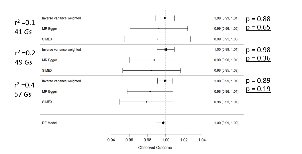The forest plot of odds ratios visualized with JASP for each correlation coefficient set. Clearly, no causal association can be found here.

Discussion

In this notebook we demonstrated the 2SMR analysis pipeline on T2D causal effect on AD. In the end, results indicated (as witnessed not only in my previous experiments, but previous MR studies on the matter [1, 2]) that T2D has no causal association with AD. Instead, it may be a probable supposition that T2D is more closely related to vascular dementia and previous associations with T2D and AD may have been due to mixed dementia cases, where pathophysiology of both AD and vascular dementia has been present in AD case study cohorts. Vascular dementia is characterized by vascular damage in the brain, and T2D has been associated with cerebrovascular lesions. The logical next step would be to study the causal association between T2D and vascular dementia.

Back to home page

koodikoira.github.io 15.6.2021

Assessment of Causal Association Between Type 2 Diabetes and Alzheimer's Disease with Mendelian Randomisation